Up to now we've discussed fairly simple measurements of amounts, counts, and labels; but time is both easier and trickier. It's simple because it always has an obvious ordering; but tricker because the units we use to measure time aren't always easy to interpret.
Units of time are measured along the 'temporal line' that may be considered to begin at the beginning and end at the end (of the universe), a time duration with an order of magnitude of 100 billion (1011) years. There are many sources for information about time, but I have distilled what I've learned in the following graphic that relates all of the important units of time. If your data are in any one unit you can use this system to convert them to any other unit.

The graphic shows how all the important time units from seconds to years relate to one another. Although the astronomical units DAYS and YEARS have been around 'forever' newer human units such as MONTHS and WEEKS are recent inventions. The graphic shows how the SECOND, which is officially defined by a constant interval, can now be the fundamental unit of temporal measurement out of which all other units can be built. The smallest units (microseconds) are just fractions of seconds; the largest units (megayears) are multiples of years. The various ways of grouping the 31,557,600 seconds that make up each year can be quite confusing.
The first challenge is to determine a zero-point for a set of time measurements, and then a measuring unit, so we can know how to represent a given instant. The Gregorian calendar sets 0 about 2000 years ago (I won't go into the complexities of Y0K!), and Excel, uses 1900-01-01 00:00 as time = 1. It doesn't matter so long as you and your audience agree that are clear about what's meant say by
2012-02-12 15:45:39.5020 EST
which is what R reported a few seconds ago. The problem is that we are not all modern astronomers or physics committed to sharing the same units and zero-points in time, so the time instant I just queried could still be interpreted by someone as December 2 2012 rather than in the
YEAR-MONTH-DAY HOUR:MINUTE:SECOND.FRACTION
that I prefer because it clearly orders the units the way we organize numbers: most significant to least signifnicant units. And this format uses 4 kinds of characters to separate the units. It's not ideal, but data reported with time measured this way is easy to convert into other units. Sign your letters however you want, but report data in something like this format.
Another challenge is to distinguish instants of time from time durations, not unlike measurements of location (3.2 kilometers from here) versus measurements of distance (a line 3.2 kilometers long). The above measurement is an instant, but also a duration, which happens to be 1,329,079,779.502 seconds from 1969-12-31 19:00:00 EST, which is fairly unambiguous.
The simplest kind of time data is a vector events, which occur at instants of time measured to the appropriate resolution. As we did before, here is a vector of times representing the days on which events occurred. We'll call this our DAY-EVENTS:
 [1]  2012-10-02  2012-11-17  2012-05-09  2012-04-11  2012-05-09
 [6]  2012-01-08  2012-09-01  2012-10-05  2012-09-15  2012-03-04
[11]  2012-10-31  2012-05-30  2012-04-12  2012-04-24  2012-01-18
[16]  2012-06-30  2012-03-16  2012-02-20  2012-09-29  2012-03-12
[21]  2012-01-15  2012-02-01  2012-06-06  2012-10-13  2012-04-02
[26]  2012-08-17  2012-08-18  2012-02-27  2012-10-10  2012-07-28
[31]  2012-07-14  2012-11-05  2012-09-08  2012-11-24  2012-11-19
[36]  2012-12-27  2012-03-16  2012-06-28  2012-08-28  2012-07-13
[41]  2012-04-16  2012-01-16  2012-01-26  2012-01-17  2012-09-01
[46]  2012-01-20  2012-03-24  2012-10-21  2012-06-26  2012-09-28
[51]  2012-09-04  2012-11-18  2012-08-08  2012-06-12  2012-09-07
[56]  2012-06-09  2012-03-29  2012-10-08  2012-12-20  2012-01-14
[61]  2012-11-29  2012-07-02  2012-01-29  2012-12-24
We can immediately see that there are 64 dates (and not only times) and that their formats appear to be in the 'proper' order YEAR-MONTH-DAY because the last number in each triplet is often greater than 12. By the 3rd measurement we can see that these measurements are not in temporal order. But as with the measurements above it's difficult to see if there is any other pattern.
Note two things; first, we have no information about sub-day measurements; e.g. the first event could have occurred any time on the day of 2012 October 2: we don't know the hour, minute, second, etc. We also don't know how long the event took to unfold; we only have a day measurement. This is not the same thing as an event enduring the whole day, just that the day 'stamp' records that an event occured on that they. If there were another event on the same day, that date, too, would be recorded.
Here's another set of events, this time occuring on a single day, organized in the HOUR:MINUTE:SECOND order that makes them easy to analyze; we'll call this our SECOND-EVENTS dataset.
 [1] 13:51:58 13:50:55 13:31:35 14:00:30 13:36:02
 [6] 14:41:46 13:46:07 13:41:35 13:04:06 14:15:49
[11] 15:02:15 13:35:21 14:18:29 13:00:26 14:13:15
[16] 12:29:44 13:21:38 15:33:35 12:49:41 12:36:10
[21] 12:30:19 12:15:15 13:29:27 15:41:17 12:42:20
[26] 15:10:48 12:06:58 12:35:50 13:27:42 14:31:54
[31] 12:16:02 15:27:52 15:38:11 13:03:47 13:20:44
[36] 14:28:58 15:19:13 14:43:14 14:47:43 15:13:54
[41] 14:03:35 16:07:34 16:38:58 16:47:10 13:00:21
[46] 12:00:07 17:15:28 17:18:27 17:19:06 11:07:24
[51] 15:53:55 16:58:13 11:01:11 17:23:07 17:26:38
[56] 10:43:25 12:00:00 15:47:37 09:54:50 16:38:47
[61] 10:08:54 17:10:21 10:44:05 17:29:05
Events are time measurements of occurrances that can occur at random times, but - by the definition I'm using, samples must be (approximately at least) regularly spaced. Someone passively records events, but they must actively sample measurements at regularly 'spaced' time intervals. Here for example are 64 equally-spaced dates throughout a year:
Samples can be of 2 kinds, and we're already familiar with these kinds of measurements. If we count the events in a sample period then we get counts, as above; while if we make measurements of some amount, then we get amounts, as above - and we know how to describe and visualize these.
First, we can bin the DAY-EVENTS into months:
Jan Feb Mar Apr May Jun Jul Aug Sep Oct Nov Dec
  9   3   6   5   3   6   4   4   8   7   6   3
in order to see which months are accounted for in the data and how often they occur. In this case we can see:
But it's not easy to see if there's any clustering within months or 'seasons.
Se can also bin the SECOND-EVENTS into hours:
hour:  00 01 02 03 04 05 06 07 08 09 10 11 12 13 14 15 16 17 18 19 20 21
count:  0  0  0  0  0  0  0  0  0  1  3  2 11 15 10 10  5  7  0  0  0  0
To see a similar kind of sample vector. In this case we see:
A cleaner way to display this vector assumes the reader knows you're not just 'hiding' the zero-count hours:
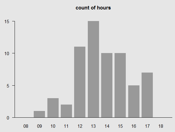
hour:  09 10 11 12 13 14 15 16 17
count:  1  3  2 11 15 10 10  5  7
In this section we have created samples simply by binning the events into convenient intervals - months and hours. We could also make measurements in each of those intervals (end-of-month bank balance, or temperature on the hour) and get very similar results.
As usual, we can order the events, which is an operation made quite easy by the proper ordering. (I leave this as an exercise...) As with phenomena, the most useful statistics are n, the number of events or samples and their range (time of the last event - time of the first).
Although it's not often done, the simplest way to visualize events is with simple marks representing the occurrance of an event. You need the minimum and maximum time instants to create the visualization. Here's a plot of each of the years from 1950 to 2014:

You can see the absolutely regular progression. Of course we don't know whether the event occured at some instant within each year, or if the period of time has been divided up into 64 periods. The first datagraphic is 'rug plot' that simply shows 64 evenly spaced events that must be controlled by some regular process. In fact, I use the term sample to refer to this kind of measurement because it reflects a controlling timer. The seccond plot shows 64 events in the same time period, but these events are clearly not happening at regularly spaced intervals. In fact, these data come from what's called a 'uniform' random number generator. This behavior is what you might find if something is occurring at unpredictable time instants.
Here is a similar plot of the DAY events. We don't know what happened before or after the year that was being monitored, but we can see the random occurrance of each of the events.
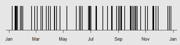
Finally, here's a plot of the SECOND events. Nothing occurs until about 10:00, then a few events arise and apparently greater frequency, then the events die out after about 18:00.

These graphics give an intuitive sense of what is going on, but we usually 'bin' events into intervals for 2 reasons: 1) the intervals smooth out some of the irregularity, and the intervals are usually human-related periods (hours, years, etc.) like the ones seen in the measurement 'flowchart' above.
If we assume that the experiment was conducted for exactly a year, beginning on 2012-jan-01 and ending on 2012-dec-31, then a natural binning system is months, which gives the following datagraphic for the random event.

And here is a plot of the hours, with (most of) the zero-count hours removed. I left the extremes just to show that we haven't 'windowed' the data.
This bar plot, which suits the visualization of binned counts, can also be used for other kinds of time series, as shown below.
So far we have examined vectors of individual events and then grouped them into convenient time periods. But if the regular time periods contain other measurements, we are dealing with time series of measurements. The next plot shows a series evenly-timed measurements one quarter apart. Notice several features:

What insights can we gain from this plot?